Sign up for breaking news, reviews, opinion, top tech deals, and more.
You are now subscribed
Your newsletter sign-up was successful
Introduction
Many of us spend a vast portion of our time banging our heads against Excel. Unfortunately we can't help you make those specific figures line up in Office 2016's spreadsheet app – that one's on you – but we can show you a few things which will make your life easier.
We're looking at tricks you can pull off inside the cells and out, improving Excel's interface while making your calculations more powerful and versatile. You'll be able to speed up data entry, change values worksheet-wide, and much more.
These tips are geared towards Excel 2016 users, and we've used Windows to pull them off, but they should all work on versions of Excel from 2010 onwards and, with the appropriate shortcut substitutions, will do the job on the Mac as well.
Article continues below- Also check out our top Word 2016 tips, along with our PowerPoint 2016 tips and Outlook 2016 tips
1. Automatic data
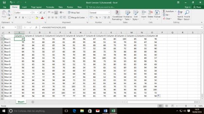
If you're preparing a spreadsheet but don't yet know what's going to go into it, you can populate its fields with random sample data before the fact to make sure your formulas are all working correctly. Click in the top left cell of the area you'd like to fill and enter the formula =RANDBETWEEN(50,100) to generate a number between 50 and 100. Change the values to suit the kind of data you'll be working with.
Now just drag the fill handle of the cell over the area you want to fill with data – it'll generate a new random number for each cell.
2. No formula fumbling
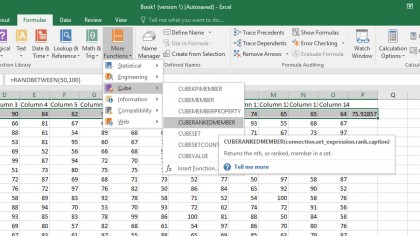
Writing your own formulas can be an arduous task, but modern versions of Excel make it far easier than it once was. Head to the Formulas tab to find the Function Library, a vast collection of all of Excel's formulas.
Click the cell in which you'd like to insert your formula, then dive in – they're all categorised, each includes a description of its function if you hover over it, and a straightforward interface in which to enter the values you want calculated.
Sign up to the TechRadar Pro newsletter to get all the top news, opinion, features and guidance your business needs to succeed!
The AutoSum function, in the same place, is a quick way to tot up figures without any typing.
3. Pasting up
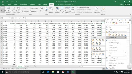
Certain formulas, like the random number generator described in our first tip, will tend to make your numbers jump around somewhat. If you'd rather keep them static, you can copy the data and, using the right click menu, paste only the generated values without the formulas. This is also a good way to distribute spreadsheets for reading without revealing your workings.
Explore the Paste Special menu to see what other kinds of paste operations you can perform: try using Paste Link to quickly create linked cells between sheets, or Transpose to paste a grid of data with the columns and rows swapped around.
4. See formulas
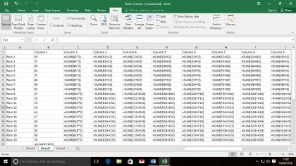
Clicking through a sheet full of numbers to find out how they've come to be is not a task many would relish. It's slow and laborious, and easy to lose track. Better, then, to use the shortcut [Ctrl]+[ ] (that's the key at the top-left of your keyboard – just below the Escape key) to show all of the formulas on your sheet instead of their result. Hit the shortcut again to switch them back.
If, for some reason, you want the sheet to show the text of a formula rather than the result of it – perhaps you're creating a demonstration sheet to show how things are meant to work – just right click the cell it's in and select Format Cells > Text.
5. Quick formatting
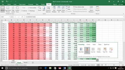
Drag to select a group of data, and look out for an icon appearing at the bottom-right hand corner of your selection area. This could be Excel's coolest feature: the quick analysis tool.
It gives you instant access to a bunch of useful formatting features, all the way from colouring up your cells based on their range to implementing sparklines, sums and charts. Hover over each option to see a preview and click it to lock it down. Use the same tool to clear formatting if it gets too much – you'll find the clear option listed under the Formatting heading.
6. Define constants
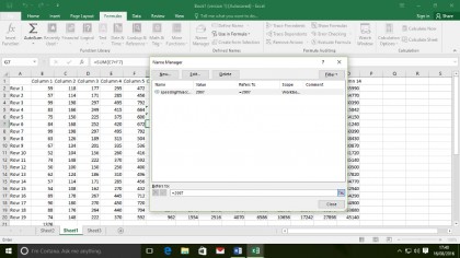
If you're a heavy Excel user, it's likely that you're running with the same figures a lot of the time. Defining a constant – representing a complex number with a short word – can speed up formula creation greatly. Head to the Formulas tab and click Define Name.
Pop the word or code you'd like to use in the uppermost box ('speedlightvacuum', for example) and the value you'd like it to represent in the bottom box (say '299792458'). Now you can just type the constant name in place of the number, preventing mistakes later on. If the speed of light in a vacuum happens to change, as it so often does, hop into the Name Manager and tweak the number – it'll change that value wherever you've used it in your workbook.
7. Keep comments
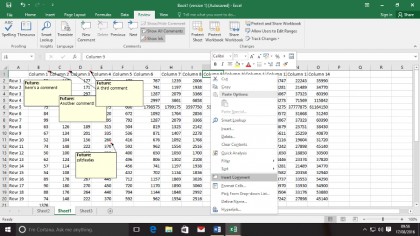
A good workbook is one that others can read and work with, without the help of the creator. Presenting someone with a complex web of numbers and expecting them to get results is just unfair. Right click a cell you'd like to explain and select Insert Comment to attach a note to that cell; you can resize and reposition the comment box if required. A cell with a comment is marked with a red flash in its top-right corner, and hovering over the cell will display that comment.
It's a good idea to add comments to column or row headers, and use the spacing tools to move them around so they're not overlapping. The Show All Comments button in the Review tab will bring them all up at once.
8. Sidestep slowdown
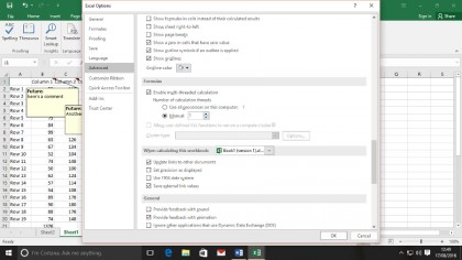
A worksheet full of formulas is a beautiful thing, but making small tweaks or running large datasets can have a big impact on the performance of your computer as a whole. To reduce the impact, you can ask Excel to use less of your processor – this will make complex formulas take longer to update, but leave the rest of your CPU open for other tasks.
Head to File > Options > Advanced and scroll down to the Formulas section. You can either disable multi-threaded calculation altogether, or use the Manual radio button to select just how many threads you want to dedicate to running your calculations.
9. Cutting corners
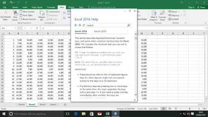
We've got a few handy shortcuts to get you working faster, now, starting with [Ctrl]+[Shift]+[$], which will automatically convert a range of numbers into whatever your default currency is. [Ctrl]+[Shift]+[#], on the other hand, converts a range of numbers into your default date format.
Holding [Ctrl] and hitting the arrow keys will jump to the end of the current row or column; hold [Shift] as well to select those cells. [Ctrl]+[Pg Up] or [Pg Down] jumps between the sheets in your current workbook. There are loads more – search 'shortcuts' in the search box to find them – but sadly there's no way to create your own custom shortcuts in the same way as Word 2016.
10. See the future
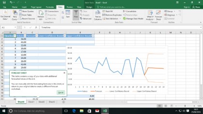
Excel now includes forecasting tools which will analyse historical data and predict future trends based on them. You'll need to begin with a key column either sorted with consecutive indices or dates so that the tool knows what order your data is in. Then select all relevant data and head to Data > Forecast sheet. Either hit Create or expand the Options menu to tweak the output.
You'll be given a line graph with Excel's average projection, and its thoughts on the potential upper or lower bounds of future figures. We wouldn't take it as gospel, but it's a useful tool to potentially extrapolate information from otherwise baffling figures.