Top ten time-saving tips – Excel
The top ten Excel tips for small business

Our top ten Excel hints and tips to make your life easier, in no particular order.
1/ Putting text on several lines
If you're typing text or multiple lines of data into a cell and you want the text to appear on several lines, then instead of entering the text in another cell just simply press
ALT+ENTER
And you'll start a new line while you're typing or editing data
2/ Add a calculator to the excel toolbar
There's a calculator in Excel 2010 but by default this feature is hidden, to get the calculator on your Excel screen navigate to Quick Access toolbar options – it's the down arrow symbol next to the undo button on the top left-hand of the screen - and click More Commands.
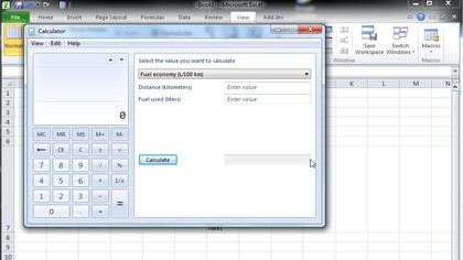
It will lead you to Excel Options dialog, under Choose commands, click drop-down button to select All Commands. Now scroll-down to find the Calculator command and click Add >> to show it in Quick Access toolbar. Hit Ok to continue
Click Calculator button in Quick Access toolbar to immediately open Calculator. Now you can use it for simple calculations
Are you a pro? Subscribe to our newsletter
Sign up to the TechRadar Pro newsletter to get all the top news, opinion, features and guidance your business needs to succeed!
3/ Changing the Enter key behaviour
When you hit the Enter key in Excel, you will automatically drop down to the
cell just below it. But you can change this default and change this feature.
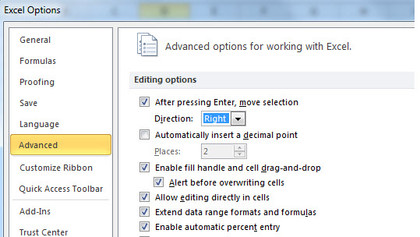
Go to Excel Options – It's found under the File tab and select options – then, select the Advanced options and under the editing options select your choice from the dropdown box.
4/ Change sheet names and colour
To give your worksheets some personalisation like month or year names instead of the "Sheet1" to "Sheet3" that Excel defaults to simply right-click on the tab and click on Rename, or double click on the worksheet tab and start typing on to the tab.
If you have lot of worksheets it's very easy to lose track of the right worksheet. To help find the right worksheet you can colour coordinate each sheet, so all 2012 monthly sales sheets could be in shades of Orange, where as 2011 sheets could be in shades of red.
To change the colour of the tab, simply right-click on the worksheet you want to change the colour of and select "Tab color" option to change the worksheet tab colours.
5/ Quickly skip through your worksheets using shortcut keys
Just as you can use ALT + TAB to skip through the opened program windows on your Windows desktop, you can do a similar thing to skip through the worksheets in Excel.
To move one worksheet to the right press
CTRL+PAGE DOWN
To move one worksheet to the left press
CTRL+PAGE UP
6/ Display Formulas Instead of Results
A single keystroke lets you toggle between Excel's normal display, which shows the results of the formulas in the spreadsheet, and a display mode that shows the actual formulas.
The keystroke is
Ctrl + '
(The grave accent key is located on the top left of the keyboard next to the 1 key, in the US it's the Tilde key); press it once, and Excel displays formulas instead of results. Press it again, and the results appear again.
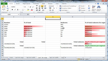
Alternatively you can achieve the same result by selecting the option to display formulas.
Open the File menu, go to Options, then Advanced;
Scroll down to Display Options for this Worksheet
Check the box next to "Show formulas in cells instead of their calculated results."
Uncheck the box if you wish to display results again.
7/ Keeping data hidden in printouts
When it's time to print your Excel worksheet, you may prefer that some information is left unprinted. For example, you may have some confidential information (such as employee salaries) in a column.
To avoid printing specific rows or columns, just hide them before printing. To hide rows, select them by clicking the row or column (click and drag to select a block of rows/columns; hold down Ctrl while clicking to select non-adjacent rows/columns). Then right-click one of the highlighted border row/columns and click Hide.
When you're finished printing, you can quickly unhide all rows or columns by selecting the entire worksheet (click the box at the top-left of the row and column borders). Then right-click a row or column border and choose Unhide.
8/ Shade Alternate Rows
For a lengthy list, shading alternate rows can improve legibility and it's simple to do with Excel's Conditional Formatting feature, which allows you to apply cell shading (green or otherwise) to every other row in a worksheet range.
Highlight the range of cells or rows or columns that you want to format.
Choose Format, Conditional Formatting to display the Conditional Formatting dialog box.
Select New Rule and then select "Use a formula to determine which cells to format," and enter
=MOD(ROW(),2)=0
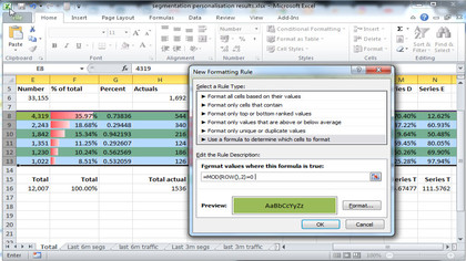
into the "Format values where this formula is true". Click the Format button to bring up the Format Cells dialog box and select the Patterns tab and specify a colour for the shaded rows. Then click Ok and the rows will be formatted in the colour of your choice.
You'll probably want to choose a light colour, so that the default black text will still be legible. Or, you can go all out and change the text colour as well (do this in the Font tab of the Format Cells dialog box).
9/ Setting up a form
Most businesses have some standard forms, timesheets, expenses forms etc and most are setup in Excel. This tip allows you set up a number of data input cells and allows the user to quickly move between input cells just by pressing the Tab key.
The key to this tip is to lock down all the cells in the spreadsheet apart from the input cells.
Select all of the input cells on your worksheet. (To select non-adjacent cells, hold down Ctrl while you select the cells.)
Select Format Cells to display the Format Cells dialog box.
Click the Protection tab and remove the check mark from the Locked check box.
Click OK.
Keep in mind that all cells are locked by default. But also remember that locking or unlocking cells has no effect unless the worksheet is protected. To protect the worksheet, select Tools, Protection, Protect Sheet.
When the sheet is protected, you'll find pressing Tab moves the active cell indicator to the next unlocked cell.
10/ Adding a drop-down list
Standard forms also tend to have standard answers, such as a day of the week, or a month, so a drop-down box with pre-filled selections would be useful.
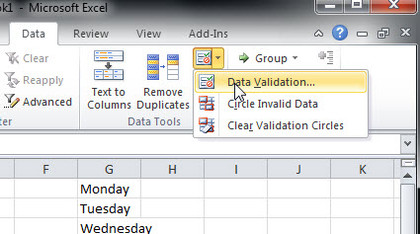
Assume that you have an input cell in which the user is supposed to enter a day of the week: Monday, Tuesday, Wednesday etc.
Enter the items for your drop-down list into a list on the worksheet, one item per cell. In this example, I'll assume that the month names start in cell G1 and extend down to G7, but normally you would put them outside of the readable area. In Excel terminology, a rectangular group of cells (such as G1 to G7) is called a range.
Select the cell that will contain the drop-down list. If you'd like more than one cell to display the same list, just select them all now rather than setting them up one at a time. (Click and drag to select a range; hold down Ctrl while you click to select non-adjacent cells.)
Select the cell where you want the drop-down list.
On the Data tab, in the Data Tools group, click Data Validation
In the Allow box, click List.
To specify the location of the list of valid entries, enter a reference to your list in the Source box in this case it's (=$G$1:$G$7) or click in the Source box and then select your list in the current spread sheet to populate the reference automatically.
Make sure that the In-cell dropdown check box is selected.
To specify whether the cell can be left blank, select or clear the Ignore blank check box.
You can go one stage further and display an input message when the cell is clicked.
Click the Error Alert tab, and make sure that the Show error alert after invalid data is entered check box is selected.
Select one of the following options for the Style box:
To display an information message that does not prevent entry of invalid data, click Information.
To display a warning message that does not prevent entry of invalid data, click Warning.
To prevent entry of invalid data, click Stop.
Type the title and text for the message (up to 225 characters).
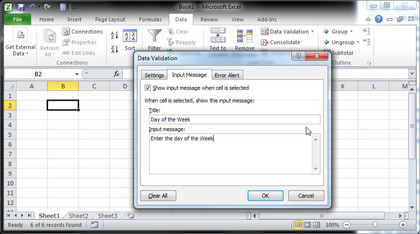
Note If you don't enter a title or text, the title defaults to "Microsoft Excel" and the message to: "The value you entered is not valid. A user has restricted values that can be entered into this cell."
After performing these steps, you'll see a drop-down arrow whenever any of the drop-down cells you just defined is "active" (that is, selected and awaiting input). Click the arrow and choose a month from the list. If you try to type something else into the cell, you'll get scolded in the form of a pop-up message.
If you'd like to provide your own wording for invalid entries, use the Error Alert tab in the Data Validation dialog box, and enter your own text in the 'Error message' field.
If your list of items is relatively small, you can enter the list items directly into the Source field. Just separate each list item with a comma.